mrc
-
hf.mrc(tick_series_list, theta=None, g=None, bias_correction=True, pairwise=True, k=None)[source]¶ The modulated realised covariance (MRC) estimator of Christensen et al. (2010).
- Parameters
- tick_series_listlist of pd.Series
Each pd.Series contains tick-log-prices of one asset with datetime index.
- thetafloat, optional, default=None
Theta is used to determine the preaveraging window
k. Ifbias_correctionis True (see below) then \(k = \theta \sqrt{n}\), else \(k = \theta n^{1/2+ 0.1}\). Hautsch & Podolskij (2013) recommend 0.4 for liquid assets and 0.6 for less liquid assets. Iftheta=0, the estimator reduces to the standard realized covariance estimator. Iftheta=Noneandkis not specified explicitly, the suggested theta of 0.4 is used.- gfunction, optional, default =
None A vectorized weighting function. If
g = None, \(g=min(x, 1-x)\)- bias_correctionboolean, optional
If
True(default) then the estimator is optimized for convergence rate but it might not be p.s.d. Alternatively as described in Christensen et al. (2010) it can be ommited. Then k should be chosen larger than otherwise optimal.- pairwisebool, default=True
If
Truethe estimator is applied to each pair individually. This increases the data efficiency but may result in an estimate that is not p.s.d.- kint, optional, default=None
The bandwidth parameter with which to preaverage. Alternative to theta. Useful for non-parametric eigenvalue regularization based on sample spliting.
- Returns
- mrcnumpy.ndarray
The mrc estimate of the integrated covariance.
Notes
The MRC estimator is the equivalent to the realized integrated covariance estimator using preaveraged returns. It is of thus of the form
\[\begin{equation} \label{eqn:mrc_raw} \left[\mathbf{Y}\right]^{(\text{MRC})}=\frac{n}{n-K+2} \frac{1}{\psi_{2} K} \sum_{i=K-1}^{n} \bar{\mathbf{Y}}_{i} \bar{\mathbf{Y}}_{i}^{\prime}, \end{equation}\]where \(\frac{n}{n-K+2}\) is a finite sample correction, and
\[\begin{split}\begin{equation} \begin{aligned} &\psi_{1}^{k}=k \sum_{i=1}^{k}\left(g\left(\frac{i}{k}\right)-g \left(\frac{i-1}{k}\right)\right)^{2}\\ &\psi_{2}^{k}=\frac{1}{k} \sum_{i=1}^{k-1} g^{2}\left(\frac{i}{k}\right). \end{aligned} \end{equation}\end{split}\]In this form, however, the estimator is biased. The bias corrected estimator is given by
\[\begin{equation} \label{eqn:mrc} \left[\mathbf{Y}\right]^{(\text{MRC})}=\frac{n}{n-K+2} \frac{1}{\psi_{2} k} \sum_{i=K-1}^{n} \bar{\mathbf{Y}}_{i} \left(\bar{\mathbf{Y}}_{i}-\frac{\psi_{1}}{\theta^{2} \psi_{2}} \hat{\mathbf{\Psi}}\right)^{\prime}, \end{equation}\]where
\[\begin{equation} \hat{\mathbf{\Psi}}=\frac{1}{2 n} \sum_{i=1}^{n} \Delta_{i}\mathbf{Y} \left(\Delta_{i} \mathbf{Y}\right)^{\prime}. \end{equation}\]The rate of convergence of this estimator is determined by the window-length \(K\). Choosing \(K=\mathcal{O}(\sqrt{n})\), delivers the best rate of convergence of \(n^{-1/4}\). It is thus suggested to choose \(K=\theta \sqrt{n}\), where \(\theta\) can be calibrated from the data. Hautsch and Podolskij (2013) suggest values between 0.4 (for liquid stocks) and 0.6 (for less liquid stocks).
Note
The bias correction may result in an estimate that is not positive semi-definite.
If positive semi-definiteness is essential, the bias-correction can be omitted. In this case, \(K\) should be chosen larger than otherwise optimal with respect to the convergence rate. Of course, the convergence rate is slower then. The optimal rate of convergence without the bias correction is \(n^{-1 / 5}\), which is attained when \(K=\theta n^{1/2+\delta}\) with \(\delta=0.1\).
thetashould be chosen between 0.3 and 0.6. It should be chosen higher if (i) the sampling frequency declines, (ii) the trading intensity of the underlying stock is low, (iii) transaction time sampling (TTS) is used as opposed to calendar time sampling (CTS). A highthetavalue can lead to oversmoothing when CTS is used. Generally the higher the sampling frequency the better. Sincemrc()andmsrc()are based on different approaches it might make sense to ensemble them. Monte Carlo results show that the variance estimate of the ensemble is better than each component individually. For covariance estimation the preaveragedhayashi_yoshida()estimator has the advantage that even ticks that don’t contribute to the covariance (due to log-summability) are used for smoothing. It thus uses the data more efficiently.References
Christensen, K., Kinnebrock, S. and Podolskij, M. (2010). Pre-averaging estimators of the ex-post covariance matrix in noisy diffusion models with non-synchronous data, Journal of Econometrics 159(1): 116–133.
Hautsch, N. and Podolskij, M. (2013). Preaveraging-based estimation of quadratic variation in the presence of noise and jumps: theory, implementation, and empirical evidence, Journal of Business & Economic Statistics 31(2): 165–183.
Examples
>>> np.random.seed(0)
>>> n = 2000
>>> returns = np.random.multivariate_normal([0, 0], [[1, 0.5],[0.5, 1]], n)
>>> returns /=  n**0.5
>>> prices = 100 * np.exp(returns.cumsum(axis=0))
>>> # add Gaussian microstructure noise
>>> noise = 10 * np.random.normal(0, 1, n * 2).reshape(-1, 2)
>>> noise *= np.sqrt(1 / n ** 0.5)
>>> prices += noise
>>> # sample n/2 (non-synchronous) observations of each tick series
>>> series_a = pd.Series(prices[:, 0]).sample(int(n/2)).sort_index()
>>> series_b = pd.Series(prices[:, 1]).sample(int(n/2)).sort_index()
>>> # take logs
>>> series_a = np.log(series_a)
>>> series_b = np.log(series_b)
>>> icov_c = mrc([series_a, series_b], pairwise=False)
>>> # This is the unbiased, corrected integrated covariance matrix estimate.
>>> np.round(icov_c, 3)
array([[0.882, 0.453],
       [0.453, 0.934]])
>>> # This is the unbiased, corrected realized variance estimate.
>>> ivar_c = mrc([series_a], pairwise=False)
>>> np.round(ivar_c, 3)
array([[0.894]])
>>> # Use ticks more efficiently by pairwise estimation
>>> icov_c = mrc([series_a, series_b], pairwise=True)
>>> np.round(icov_c, 3)
array([[0.894, 0.453],
       [0.453, 0.916]])
