krvm
-
hf.krvm(tick_series_list, H, pairwise=True, kernel=CPUDispatcher(<function quadratic_spectral_kernel at 0x7f36d4bb61e0>))[source]¶ The kernel realized volatility matrix estimator (KRVM) of Barndorff-Nielsen et al. (2011).
- Parameters
- tick_series_listlist of pd.Series
Each pd.Series contains tick-log-prices of one asset with datetime index.
- Hint, > 0
The bandwidth parameter for the Parzen kernel. Should be on the order of \(n^{3/5}\).
- pairwisebool, default=True
If
Truethe estimator is applied to each pair individually. This increases the data efficiency but may result in an estimate that is not p.s.d even for the p.s.d version of thiss estimator.- kernelfunction, default=quadratic_spectral_kernel
The kernel weighting function.
- Returns
- covnumpy.ndarray
The intgrated covariance matrix estimate.
Notes
The multivariate realized kernel estimator smoothes the autocovariance operator and thereby achieves the optimal convergence rate in the multivariate setting with noise and asynchronous observation times. Incidentally, this estimator is similar in form to the HAC, widely used in the statistics and econometrics literature to deal with heteroscedastic and autocorrelated noise. Observations are synchronized with the
refresh-time()scheme. In addition, \(m\) observation are averaged at the beginning and at the end of the trading day to estimate the efficient price at these times. The authors call this ‘jittering’. In practice the effect of jittering is negligible but it is needed for proving consistency. (It is ignored in this implementation.) The, with parameter \(m\), jittered log-price vectors are denoted as \(\mathbf{Y}^{(m)}(s), s=1, \ldots, n-2 m+1\). The kernel estimator is defined by \begin{equation} \widehat{\mathbf{\Sigma}}^{(KRVM)}=\boldsymbol{\gamma}^{(0)} \left(\mathbf{Y}^{(m)}\right)+\sum_{h=1}^{n-2 m} k\left(\frac{h-1}{H} \right)\left[\boldsymbol{\gamma}^{(h)}\left(\mathbf{Y}^{(m)}\right)+ \boldsymbol{\gamma}^{(-h)}\left(\mathbf{Y}^{(m)}\right)\right], \end{equation} where \begin{equation} \boldsymbol{\gamma}^{(h)}\left(\mathbf{Y}\right)= \sum_{s=h+2}^{n+1}\left(\mathbf{Y}(s)-\mathbf{Y}(s-1)\right) \left(\mathbf{Y}(s-h)-\mathbf{Y}(s-h-1)\right)^{\prime}, \quad h \geq 0 \end{equation} and \begin{equation} \boldsymbol{\gamma}^{(h)}\left(\mathbf{Y}\right)= \boldsymbol{\gamma}^{(-h)}\left(\mathbf{Y}\right)^{\prime}, \quad h < 0, \end{equation} with \(\mathbf{Y}\) denoting the synchronized zero-return log-price. \(\boldsymbol{\gamma}^{(h)}\) is the \(h\)th realized autocovariance (gamma()). \(k(\cdot)\) is the kernel function with its bandwidth parameter \(H\). It is assumed that (i) \(k(0)=1\) and \(k^{\prime}(0)=0\), (ii) \(k(\cdot)\) is twice differentiable with continuous derivatives, and (iii) \(\int_{0}^{\infty} k(x)^{2} d x, \int_{0}^{\infty} k^{\prime}(x)^{2} d x\) and \(\int_{0}^{\infty} k^{\prime \prime}(x)^{2} d x\) are finite. A slightly adjusted form of this estimator that is positive semidefinite is given by \begin{equation} \widehat{\mathbf{\Sigma}}^{(KRVM_{psd})}=\boldsymbol{\gamma}^{(0)} \left(\mathbf{Y}^{(m)}\right)+\sum_{h=1}^{n-2 m} k\left(\frac{h}{H}\right) \left[\boldsymbol{\gamma}^{(h)}\left(\mathbf{Y}^{(m)}\right)+ \boldsymbol{\gamma}^{(-h)}\left(\mathbf{Y}^{(m)}\right)\right]. \end{equation} This form requires the additional assumption \(\int_{-\infty}^{\infty} k(x) \exp (i x \lambda) d x \geq 0\) for all \(\lambda \in \mathbb{R}\).Choosing the right kernel function is important. The authors show, for example, that the estimator based on the Bartlett weight function is inconsistent. Instead, the Parzen kernel (
parzen_kernel()) is suggested as a weight function that yields a consistent estimator and can be efficiently implemented. The bandwidth \(H\) must be on the order of \(n^{3 / 5}\). The authors choose the scalar \(H\) as the average of optimal individual \(H^{(j)}\): $$\bar{H}=p^{-1} \sum_{j=1}^{p} H^{(j)},$$ where \begin{equation} H^{(j)}=c^{*} \xi_{j}^{4 / 5} n^{3 / 5}, \end{equation} with \begin{equation} c^{*}=\left\{k^{\prime \prime}(0)^{2} / k_{\bullet}^{0,0}\right\}^{1 / 5}, \end{equation} and \begin{equation} \xi_{j}^{2}={\Sigma}_{\epsilon, j j} / {\Sigma}_{j j}. \end{equation} \(\mathbf{\Sigma}_{\epsilon}\) and \(\mathbf{\Sigma}\) denote, as previously defined, the integrated covariance matrix of the noise and the efficient return process, respectively. Here these quantities are understood over the interval under consideration. Hence, \(\xi_{j}^{2}\) can be interpreted as the ratio of the noise variance and the return variance. For the Parzen kernel \(c^{*} = 3.51\), as tabulated by the authors. It is a measure of the relative asymptotic efficiency of the kernel. \({\Sigma}_{j j}\) may be estimated via a low frequency estimator and \({\Sigma}_{\epsilon,j j}\) via a high frequency estimator.References
Barndorff-Nielsen, O. E., Hansen, P. R., Lunde, A. and Shephard, N. (2011). Multivariate realised kernels: consistent positive semi-definite estimators of the covariation of equity prices with noise and non-synchronous trading, Journal of Econometrics 162(2): 149– 169.
