hayashi_yoshida
-
hf.hayashi_yoshida(tick_series_list, theta=None, k=None)[source]¶ The (pairwise) Hayashi-Yoshida estimator of Hayashi and Yoshida (2005). This estimtor sums up all products of time-overlapping returns between two assets. This makes it possible to compute unbiased estimates of the integrated covariance between two assets that are sampled non-synchronously. The standard realized covariance estimator is biased toward zero in this case. This is known as the Epps effect. The function is accelerated via JIT compilation with Numba. The preaveraged version handles microstructure noise as shown in Christensen et al. (2010).
- Parameters
- tick_series_listlist of pd.Series
Each pd.Series contains tick-log-prices of one asset with datetime index.
- thetafloat, theta>=0, default=None
If
theta=Noneandkis not specified explicitly, theta will be set to 0. If theta>0, the log-returns are preaveraged with theta and \(g(x) = min(x, 1-x)\). Hautsch and Podolskij (2013) suggest values between 0.4 (for liquid stocks) and 0.6 (for less liquid stocks). Iftheta=0, this is the standard HY estimator.- kint, >=1, default=None
The bandwidth parameter with which to preaverage. Alternative to
theta. Useful for non-parametric eigenvalue regularization based on sample splitting. Whenk=Noneandtheta=None,kwill be set to 1. Ifk=1, this is the standard HY estimator.
- Returns
- covnumpy.ndarray
The pairwise HY estimate of the integrated covariance matrix.
Notes
The estimator is defined as
\[\begin{equation} \left\langle X^{(k)}, X^{(l)}\right\rangle_{H Y}= \sum_{i=1}^{n^{(k)}}\sum_{i'=1}^{n^{(l)}} \Delta X_{t^{(k)}_i}^{(k)} \Delta X_{t^{(l)}_{i^{\prime}}}^{(l)} \mathbf{1}_{\left\{\left(t_{i-1}^{(k)}, t_{i}^{(k)}\right] \cap\left(t_{i^{\prime}-1}^{(l)}, t_{i^{\prime}}^{(l)}\right]\neq \emptyset \right\}}, \end{equation}\]where
\[\Delta X_{t^{(j)}_i}^{(j)} :=X_{t^{(j)}_i}^{(j)} - X_{t^{(j)}_{i-1}}^{(j)}\]denotes the jth asset tick-to-tick log-return over the interval spanned from
\[{t^{(j)}_{i-1}} \text{ to } {t^{(j)}_i}, i = 1, \cdots, n^{(j)}.\]and \(n^{(j)} = |t^{(j)}| -1\) denotes the number of tick-to-tick returns. The following diagram visualizes the products of returns that are part of the sum by the dashed lines.
![\draw (0,1.75) -- (11,1.75)
(0,-0.75) -- (11,-0.75)
(0,1.5) -- (0,2)
(1.9,1.5) -- (1.9,2)
(4,1.5) -- (4,2)
(5,1.5) -- (5,2)
(7.3,1.5) -- (7.3,2)
(10.8,1.5) -- (10.8,2)
(0,-0.5) -- (0,-1)
(1.9,-0.5) -- (1.9,-1)
(5.7,-0.5) -- (5.7,-1)
(8,-0.5) -- (8,-1)
(10.3,-0.5) -- (10.3,-1);
\draw[dashed,gray]
(1.1,1.75) -- (1.1,-0.75)
(3,1.75) -- (3.8,-0.75)
(4.5,1.75) -- (3.8,-0.75)
(6.15,1.75) -- (3.8,-0.75)
(6.15,1.75) -- (6.8,-0.75) ;
\draw[dashed] (11,1.75) -- (12,1.75)
(11,-0.75) -- (12,-0.75);
\draw[very thick] (9.5,-1.4) -- (9.5,0.25)
(9.5,0.8) -- (9.5,2.4);
\draw (0,0.5) node{$t_{0}^{(k)}=t_{0}^{(l)}=0$}
(1.9,1) node{$t_{1}^{(k)}$}
(4,1) node{$t_{2}^{(k)}$}
(5,1) node{$t_{3}^{(k)}$}
(7.3,1) node{$t_{4}^{(k)}$}
(11,1) node{$t_{5}^{(k)}$}
(9.5,0.5) node{\textbf{$T$}}
(1.9,0) node{$t_{1}^{(l)}$}
(5.7,0) node{$t_{2}^{(l)}$}
(8,0) node{$t_{3}^{(l)}$}
(10.3,0) node{$t_{4}^{(l)}$};
\draw (0,1.75) node[left,xshift=-0pt]{$X^{(k)}$}
(0,-0.75) node[left,xshift=-0pt]{$X^{(l)}$};
\draw[decorate,decoration={brace,amplitude=12pt}]
(0,2)--(1.9,2) node[midway, above,yshift=10pt,]
{$ \Delta X_{t^{(k)}_1}^{(k)}$};
\draw[decorate,decoration={brace,amplitude=12pt}]
(1.9,2)--(4,2) node[midway, above,yshift=10pt,]
{$ \Delta X_{t^{(k)}_2}^{(k)}$};
\draw[decorate,decoration={brace,amplitude=12pt}]
(4,2)--(5,2) node[midway, above,yshift=10pt,]
{$ \Delta X_{t^{(k)}_3}^{(k)}$};
\draw[decorate,decoration={brace,amplitude=12pt}]
(5,2)--(7.3,2) node[midway, above,yshift=10pt,]
{$ \Delta X_{t^{(k)}_4}^{(k)}$};
\draw[decorate,decoration={brace,amplitude=12pt}]
(8,-1)--(5.7,-1) node[midway, below,yshift=-10pt,]
{$ \Delta X_{t^{(l)}_3}^{(l)}$};
\draw[decorate,decoration={brace,amplitude=12pt}]
(5.7,-1)--(1.9,-1) node[midway, below,yshift=-10pt,]
{$ \Delta X_{t^{(l)}_2}^{(l)}$};
\draw[decorate,decoration={brace,amplitude=12pt}]
(1.9,-1)--(0,-1) node[midway, below,yshift=-10pt,]
{$ \Delta X_{t^{(l)}_1}^{(l)}$};](../_images/tikz-39845fb9a3e2c05505ef4820e3d36002e97a034c.png)
When returns are preaveraged with
preaverage(), the HY estimator of can be made robust to microstructure noise as well. It is then of the slightly adjusted form\[\begin{equation} \left\langle X^{(k)}, X^{(l)}\right \rangle_{H Y}^{\theta}=\frac{1}{ \left(\psi_{H Y} K \right)^{2}} \sum_{i=K}^{n^{(k)}} \sum_{i'=K}^{n^{(l)}} \bar{Y}_{t^{(k)}_i}^{(k)}\bar{Y}_{t^{(l)}_{i'}}^{(l)} \mathbf{1}_{\left\{\left(t_{i-K}^{(k)}, t_{i}^{(k)}\right] \cap\left(t_{i'-K}^{(l)}, t_{i'}^{(l)}\right] \neq \emptyset\right)} \end{equation}\]where \(\psi_{HY}=\frac{1}{K} \sum_{i=1}^{K-1} g\left(\frac{i}{K}\right)\) The preaveraged HY estimator has optimal convergence rate \(n^{-1/4}\), where \(n=\sum_{j=1}^{p} n^{(j)}\). Christensen et al. (2013) subsequently proof a central limit theorem for this estimator and show that it is robust to some dependence structure of the noise process. Since preaveraging is performed before synchronization, the estimator utilizes more data than other methods that cancel noise after synchronization. In particular, the preaveraged HY estimator even uses the observation \(t^{(j)}_2\) in the figure, which does not contribute the the covariance due to the log-summability.
References
Hayashi, T. and Yoshida, N. (2005). On covariance estimation of non-synchronously observed diffusion processes, Bernoulli 11(2): 359–379.
Christensen, K., Kinnebrock, S. and Podolskij, M. (2010). Pre-averaging estimators of the ex-post covariance matrix in noisy diffusion models with non-synchronous data, Journal of Econometrics 159(1): 116–133.
Hautsch, N. and Podolskij, M. (2013). Preaveraging-based estimation of quadratic variation in the presence of noise and jumps: theory, implementation, and empirical evidence, Journal of Business & Economic Statistics 31(2): 165–183.
Christensen, K., Podolskij, M. and Vetter, M. (2013). On covariation estimation for multivariate continuous itˆo semimartingales with noise in non-synchronous observation schemes, Journal of Multivariate Analysis 120: 59–84.
Examples
>>> np.random.seed(0)
>>> n = 10000
>>> returns = np.random.multivariate_normal([0, 0], [[1,0.5],[0.5,1]], n)/n**0.5
>>> prices = np.exp(returns.cumsum(axis=0))
>>> # sample n/2 (non-synchronous) observations of each tick series
>>> series_a = pd.Series(prices[:, 0]).sample(int(n/2)).sort_index()
>>> series_b = pd.Series(prices[:, 1]).sample(int(n/2)).sort_index()
>>> # take logs
>>> series_a = np.log(series_a)
>>> series_b = np.log(series_b)
>>> icov = hayashi_yoshida([series_a, series_b])
>>> np.round(icov, 3)
array([[0.983, 0.512],
       [0.512, 0.99 ]])
