msrc
-
hf.msrc(tick_series_list, M=None, N=None, pairwise=True)[source]¶ The multi-scale realized volatility (MSRV) estimator of Zhang (2006). It is extended to multiple dimensions following Zhang (2011). If
pairwise=Trueestimate correlations with pairwise-refresh time previous ticks and variances with all available ticks for each asset.- Parameters
- tick_series_listlist of pd.Series
Each pd.Series contains tick-log-prices of one asset with datetime index. Must not contain nans.
- Mint, >=1, default=None
The number of scales If
M=Noneall scales \(i = 1, ..., M\) are used, where M is chosen \(M = n^{1/2}\) acccording to Eqn (34) of Zhang (2006).- Nint, >=0, default=None
The constant \(N\) of Tao et al. (2013) If
N=None\(N = n^{1/2}\). Lam and Qian (2019) need \(N = n^{2/3}\) for non-sparse integrated covariance matrices, in which case the rate of convergence reduces to \(n^{1/6}\).- pairwisebool, default=True
If
Truethe estimator is applied to each pair individually. This increases the data efficiency but may result in an estimate that is not p.s.d.
- Returns
- outnumpy.ndarray
The mrc estimate of the integrated covariance matrix.
Notes
Realized variance estimators based on multiple scales exploit the fact that the proportion of the observed realized variance over a specified interval due to microstructure noise increases with the sampling frequency, while the realized variance of the true underlying process stays constant. The bias can thus be corrected by subtracting a high frequency estimate, scaled by an optimal weight, from a medium frequency estimate. The weight is chosen such that the large bias in the high frequency estimate, when scaled by the weight, is exactly equal to the medium bias, and they cancel each other out as a result.
By considering \(M\) time scales, instead of just two as in
tsrc(), Zhang2006 improves the rate of convergence to \(n^{-1 / 4}\). This is the best attainable rate of convergence in this setting. The proposed multi-scale realized volatility (MSRV) estimator is defined as \begin{equation} \langle\widehat{X^{(j)}, X^{(j)}}\rangle^{(MSRV)}_T=\sum_{i=1}^{M} \alpha_{i}[Y^{(j)}, Y^{(j)}]^{\left(K_{i}\right)}_T \end{equation} where \(\alpha_{i}\) are weights satisfying \begin{equation} \begin{aligned} &\sum \alpha_{i}=1\ &\sum_{i=1}^{M}\left(\alpha_{i} / K_{i}\right)=0 \end{aligned} \end{equation} The optimal weights for the chosen number of scales \(M\), i.e., the weights that minimize the noise variance contribution, are given by \begin{equation} a_{i}=\frac{K_{i}\left(K_{i}-\bar{K}\right)} {M \operatorname{var}\left(K\right)}, \end{equation} where %\(\bar{K}\) denotes the mean of \(K\). $$\bar{K}=\frac{1}{M} \sum_{i=1}^{M} K_{i} \quad \text { and } \quad \operatorname{var}\left(K\right)=\frac{1}{M} \sum_{i=1}^{M} K_{i}^{2}-\bar{K}^{2}. $$ If all scales are chosen, i.e., \(K_{i}=i\), for \(i=1, \ldots, M\), then \(\bar{K}=\left(M+1\right) / 2\) and \(\operatorname{var}\left(K\right)= \left(M^{2}-1\right) / 12\), and hence\begin{equation} a_{i}=12 \frac{i}{M^{2}} \frac{i / M-1 / 2-1 / \left(2 M\right)}{1-1 / M^{2}}. \end{equation} In this case, as shown by the author in Theorem 4, when \(M\) is chosen optimally on the order of \(M=\mathcal{O}(n^{1/2})\), the estimator is consistent at rate \(n^{-1/4}\).
References
Zhang, L. (2006). Efficient estimation of stochastic volatility using noisy observations: A multi-scale approach, Bernoulli 12(6): 1019–1043.
Zhang, L. (2011). Estimating covariation: Epps effect, microstructure noise, Journal of Econometrics 160.
Examples
>>> np.random.seed(0)
>>> n = 200000
>>> returns = np.random.multivariate_normal([0, 0], [[1,0.5],[0.5,1]], n)/n**0.5
>>> prices = 100*np.exp(returns.cumsum(axis=0))
>>> # add Gaussian microstructure noise
>>> noise = 10*np.random.normal(0, 1, n*2).reshape(-1, 2)*np.sqrt(1/n**0.5)
>>> prices +=noise
>>> # sample n/2 (non-synchronous) observations of each tick series
>>> series_a = pd.Series(prices[:, 0]).sample(int(n/2)).sort_index()
>>> series_b = pd.Series(prices[:, 1]).sample(int(n/2)).sort_index()
>>> # get log prices
>>> series_a = np.log(series_a)
>>> series_b = np.log(series_b)
>>> icov = msrc([series_a, series_b], M=1, pairwise=False)
>>> icov_c = msrc([series_a, series_b])
>>> # This is the biased, uncorrected integrated covariance matrix estimate.
>>> np.round(icov, 3)
array([[11.553,  0.453],
       [ 0.453,  2.173]])
>>> # This is the unbiased,  corrected integrated covariance matrix estimate.
>>> np.round(icov_c, 3)
array([[0.985, 0.392],
       [0.392, 1.112]])
