tsrc
-
hf.tsrc(tick_series_list, J=1, K=None)[source]¶ The two-scales realized volatility (TSRV) of Zhang et al. (2005). It is extentended to handle multiple dimension according to Zhang (2011).
msrc()has better convergence rate and is thus prefrerred.- Parameters
- tick_series_listlist of pd.Series
Each pd.Series contains tick-log-prices of one asset with datetime index.
- Kint, default =
int(n**(2/3)) long scale, default =
int(n**(2/3))as per Zhang (2005)- Jint, default = 1
short scale
- Returns
- outnumpy.ndarray
The TSRV estimate.
Notes
The two-scales realized volatility (TSRV) estimator is defined as
\begin{equation} \widehat{\langle X^{(j)}, X^{(j)}\rangle}^{(\mathrm{TSRV})}_{T}= \left[Y^{(j)}, Y^{(j)}\right]_{T}^{(K)}-\frac{\bar{n}_{K}}{\bar{n}_{J}} \left[Y^{(j)}, Y^{(j)}\right]_{T}^{(J)}, \end{equation} where \begin{equation} \left[Y^{(j)}, Y^{(j)}\right]_{T}^{(K)}=\frac{1}{K} \sum_{i=K}^{n}\left(Y_{\tau_{i}^{(j)}}^{(j)}- Y_{\tau_{i-K}^{(j)}}^{(j)}\right)^2, \end{equation} with \(K\) being a positive integer usually chosen much larger than 1 and \(\bar{n}_{K}=\left(n-K+1\right)/K\) and \(\bar{n}_{J}=\left(n- J+1\right)/J\). If \(K\) is chosen on the order of\(K=\mathcal{O}\left(n^{2 / 3}\right)\) this estimator is asymptotically unbiased, consistent, asymptotically normal distributed and converges at rate \(n^{-1 / 6}\).
Zhang (2011) proposes the (multivariate) two scales realized covariance (TSCV) estimator based on previous-tick times of asset \(k\) and \(l\), which simultaneously corrects for the bias due to asynchronicity and the bias due to microstructure noise. Previous-tick times may be computed via
refresh_time().The TSCV estimator is defined as \begin{equation} \widehat{\langle X^{(k)},X^{(l)}\rangle}_{T}^{(TSCV)}=c\left(\left[Y^{(k)}, Y^{(l)}\right]_{T}^{(K)}-\frac{\bar{n}_{K}}{\bar{n}_{J}}\left[Y^{(k)}, Y^{(l)}\right]_{T}^{(J)}\right), \end{equation} where \begin{equation} \left[Y^{(k)}, Y^{(l)}\right]_{T}^{(K)}=\frac{1}{K} \sum_{i=K}^{\tilde{n}}\left(Y^{(k)}_{\tau^{(k)}_{i}}-Y^{(k)}_{\tau^{(k)}_{i-K}} \right)\left(Y^{(l)}_{\tau^{(l)}_{i}}-Y^{(l)}_{\tau^{(l)}_{i-K}}\right) \end{equation} \(c=1+o_{p}\left(\tilde{n}^{-1 / 6}\right)\) is a small sample correction. \(K\) is again a positive integer usually chosen much larger than 1 and \(\bar{n}_{K}=\left(\tilde{n}- K+1\right) / K\) and \(\bar{n}_{J}= \left(\tilde{n}- J+1\right) / J\). The author shows that if \(K=\mathcal{O}\left((n^{(k)}+n^{(l)})^{2/3}\right)\) this estimator is asymptotically unbiased, consistent, asymptotically normal distributed and converges at rate \(\tilde{n}^{-1 / 6}\).
Note
Use
msrc()since it has better converges rate.References
Zhang, L., Mykland, P. A. and Ait-Sahalia, Y. (2005). A tale of two time scales: Determining integrated volatility with noisy high-frequency data, Journal of the American Statistical Association 100(472): 1394–1411.
Zhang, L. (2011). Estimating covariation: Epps effect, microstructure noise, Journal of Econometrics 160.
Examples
>>> np.random.seed(0)
>>> n = 200000
>>> returns = np.random.multivariate_normal([0, 0], [[1, 0.5],[0.5, 1]], n)/n**0.5
>>> prices = 100*np.exp(returns.cumsum(axis=0))
>>> # add Gaussian microstructure noise
>>> noise = 10*np.random.normal(0, 1, n*2).reshape(-1, 2)*np.sqrt(1/n**0.5)
>>> prices += noise
>>> # sample n/2 (non-synchronous) observations of each tick series
>>> series_a = pd.Series(prices[:, 0]).sample(int(n/2)).sort_index()
>>> series_b = pd.Series(prices[:, 1]).sample(int(n/2)).sort_index()
>>> # take logs
>>> series_a = np.log(series_a)
>>> series_b = np.log(series_b)
>>> icov_c = tsrc([series_a, series_b])
>>> # This is the unbiased,  corrected integrated covariance matrix estimate.
>>> np.round(icov_c, 3)
array([[0.995, 0.361],
       [0.361, 0.977]])
