nonlinear_shrinkage

hd.nonlinear_shrinkage(X)

Compute the shrunk sample covariance matrix with the analytic nonlinear shrinkage formula of Ledoit and Wolf (2018). This estimator shrinks the sample sample covariance matrix with _nonlinear_shrinkage_cov(). The code has been adapted from the Matlab implementation provided by the authors in Appendix D.

Parameters

xnumpy.ndarray, shape = (p, n)

A sample of synchronized log-returns.

Returns

sigmatildenumpy.ndarray, shape = (p, p)

The nonlinearly shrunk covariance matrix estimate.

Notes

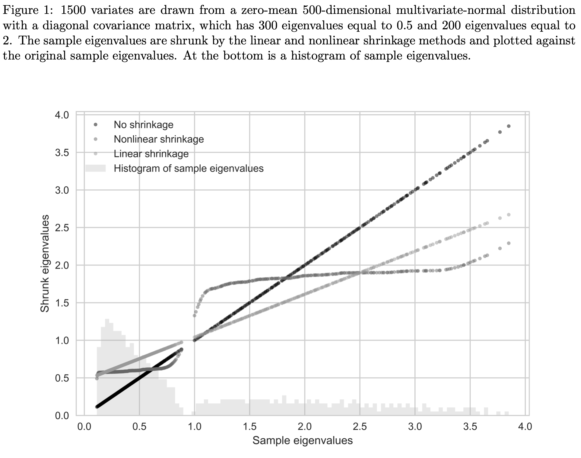
The idea of shrinkage covariance estimators is further developed by Ledoit and Wolf (2012) who argue that given a sample of size \(\mathcal{O}(p^2)\), estimating \(\mathcal{O}(1)\) parameters, as in linear shrinkage, is precise but too restrictive, while estimating \(\mathcal{O}(p^2)\) parameters, as in the the sample covariance matrix, is impossible. They argue that the optimal number of parameters to estimate is \(\mathcal{O}(p)\). Their proposed non-linear shrinkage estimator uses exactly \(p\) parameters, one for each eigenvalue, to regularize each eigenvalue with a specific shrinkage intensity individually. Linear shrinkage, in contrast, is restricted by a single shrinkage intensity with which all eigenvalues are shrunk uniformly. Nonlinear shrinkage enables a nonlinear fit of the shrunk eigenvalues, which is appropriate when there are clusters of eigenvalues. In this case, it may be optimal to pull a small eigenvalue (i.e., an eigenvalue that is below the grand mean) further downwards and hence further away from the grand mean. Linear shrinkage, in contrast, always pulls a small eigenvalue upwards. Ledoit and Wolf (2018) find an analytic formula based on the Hilbert transform that nonlinearly shrinks eigenvalues asymptotically optimally with respect to the MV-loss function (as well as the quadratic Frobenius loss). The shrinkage function via the Hilbert transform can be interpreted as a local attractor. Much like the gravitational field extended into space by massive objects, eigenvalue clusters exert an attraction force that increases with the mass (i.e. the number of eigenvalues in the cluster) and decreases with the distance. If an eigenvalue \(\lambda_i\) has many neighboring eigenvalues slightly smaller than itself, the exerted force on \(\lambda_i\) will have large magnitude and downward direction. If \(\lambda_i\) has many neighboring eigenvalues slightly larger than itself, the exerted force on \(\lambda_i\) will also have large magnitude but upward direction. If the neighboring eigenvalues are much larger or much smaller than \(\lambda_i\) the magnitude of the force on \(\lambda_i\) will be small. The nonlinear effect this has on the shrunk eigenvalues can be seen in the figure below. The linearly shrunk eigenvalues, on the other hand, follow a line. Both approaches reduce the dispersion of eigenvalues and hence deserve the name shrinkage.

The authors assume that there exists a \(n \times p\) matrix \(\mathbf{Z}\) of i.i.d. random variables with mean zero, variance one, and finite 16th moment such that the matrix of observations \(\mathbf{X}:=\mathbf{Z} \mathbf{\Sigma}^{1/2}\). Neither \(\mathbf{\Sigma}^{1/2}\) nor \(\mathbf{Z}\) are observed on their own. This assumption might not be satisfied if the data generating process is a factor model. 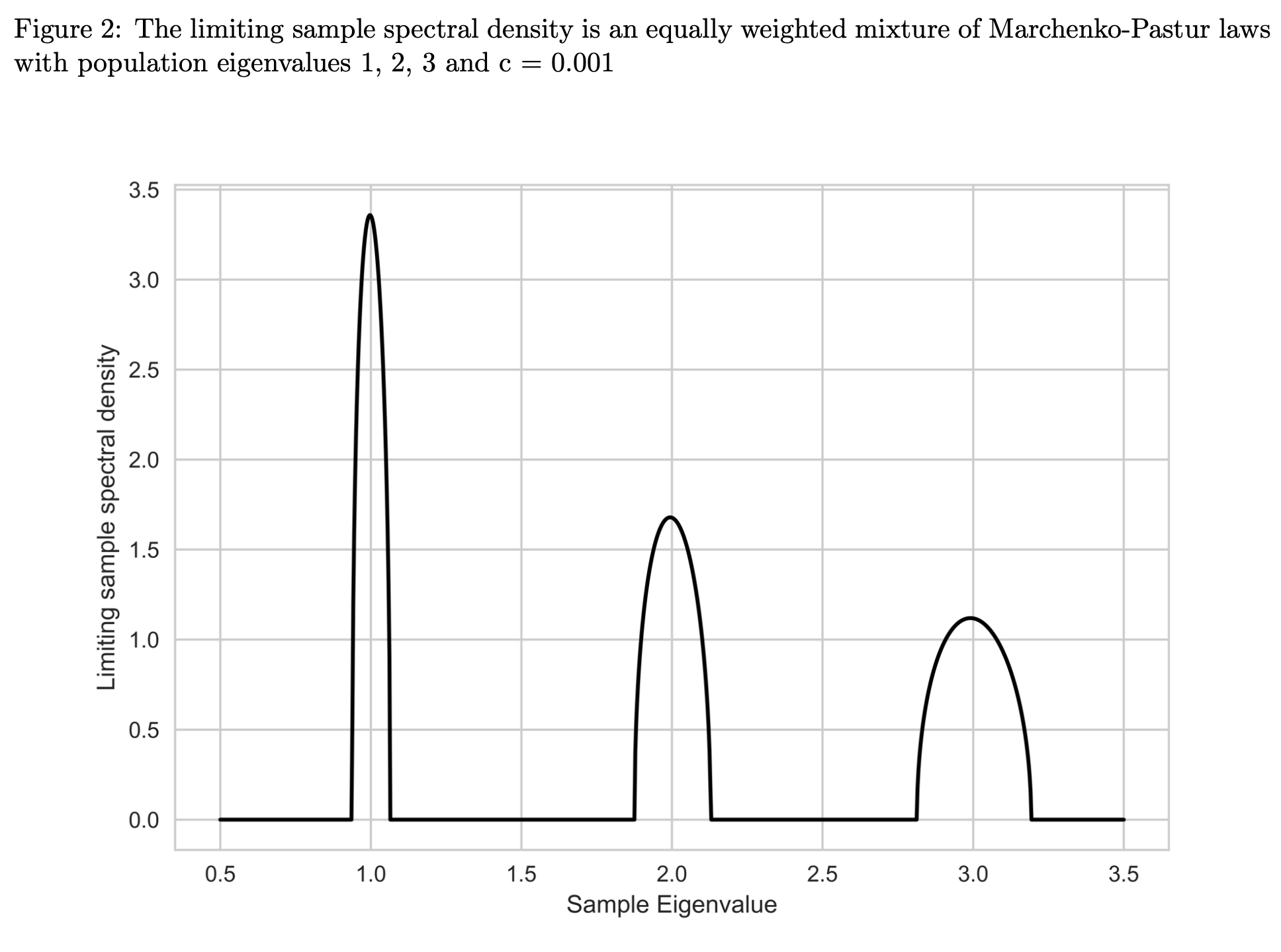Use nercome() or nerive() if you believe the assumption is in your dataset violated. Theorem 3.1 of Ledoit and Wolf (2018) states that under their assumptions and general asymptotics the MV-loss is minimized by a rotation equivariant covariance estimator, where the elements of the diagonal matrix are \begin{equation} \label{eqn: oracle diag} \widehat{\mathbf{\delta}}^{(o, nl)}:=\left(\widehat{d}_{1}^{(o, nl)}, \ldots, \widetilde{d}_{p}^{(o, nl)}\right):=\left(d^{(o, nl)}\left( \lambda_{1}\right), \ldots, d^{(o, nl)}\left(\lambda_{p}\right)\right). \end{equation} \(d^{(o, nl)}(x)\) denotes the oracle nonlinear shrinkage function and it is defined as \begin{equation} \forall x \in \operatorname{Supp}(F) \quad d^{(o, nl)}(x):=\frac{x}{ [\pi c x f(x)]^{2}+\left[1-c-\pi c x \mathcal{H}_{f}(x)\right]^{2}}, \end{equation} where \(\mathcal{H}_{g}(x)\) is the Hilbert transform. As per Definition 2 of Ledoit and Wolf (2018) it is defined as \begin{equation} \forall x \in \mathbb{R} \quad \mathcal{H}_{g}(x):=\frac{1}{\pi} P V \int_{-\infty}^{+\infty} g(t) \frac{d t}{t-x}, \end{equation} which uses the Cauchy Principal Value, denoted as \(PV\) to evaluate the singular integral in the following way \begin{equation} P V \int_{-\infty}^{+\infty} g(t) \frac{d t}{t-x}:=\lim _{\varepsilon \rightarrow 0^{+}}\left[\int_{-\infty}^{x-\varepsilon} g(t) \frac{d t} {t-x}+\int_{x+\varepsilon}^{+\infty} g(t) \frac{d t}{t-x}\right]. \end{equation} It is an oracle estimator due to the dependence on the limiting sample spectral density \(f\), its Hilbert transform \(\mathcal{H}_f\), and the limiting concentration ratio \(c\), which are all unobservable. Nevertheless, it represents progress compared to hd.fsopt(), since it no longer depends on the full population covariance matrix, \(\mathbf{\Sigma}\), but only on its eigenvalues. This reduces the number of parameters to be estimated from the impossible \(\mathcal{O}(p^2)\) to the manageable \(\mathcal{O}(p)\). To make the estimator feasible, unobserved quantities have to be replaced by statistics. A consistent estimator for the limiting concentration \(c\) is the sample concentration \(c_n = p/n\). For the limiting sample spectral density \(f\), the authors propose a kernel estimator. This is necessary, even though \(F_{n}\stackrel{\text { a.s }}{\rightarrow} F\), since \(F_n\) is discontinuous at every \(\lambda_{i}\) and thus its derivative \(f_n\), which would’ve been the natural estimator for \(f\), does not exist there. A kernel density estimator is a non-parametric estimator of the probability density function of a random variable. In kernel density estimation data from a finite sample is smoothed with a non-negative function \(K\), called the kernel, and a smoothing parameter \(h\), called the bandwidth, to make inferences about the population density. A kernel estimator is of the form \begin{equation} \widehat{f}_{h}(x)=\frac{1}{N} \sum_{i=1}^{N} K_{h}\left(x-x_{i}\right)= \frac{1}{N h} \sum_{i=1}^{N} K\left(\frac{x-x_{i}}{h}\right). \end{equation}

The chosen kernel estimator for the limiting sample spectral density is based on the Epanechnikov kernel with a variable bandwidth, proportional to the eigenvalues, \(h_{i}:=\lambda_{i} h,\) for \(i=1, \ldots, p\), where the global bandwidth is set to \(h:=n^{-1 / 3}\). The reasoning behind the variable bandwidth choice can be intuited from the figure below, which shows that the support of the limiting sample spectral distribution is approximately proportional to the eigenvalue.

The Epanechnikov kernel is defined as \begin{equation} \forall x \in \mathbb{R} \quad \kappa^{(E)}(x):= \frac{3}{4 \sqrt{5}}\left[1-\frac{x^{2}}{5}\right]^{+}. \end{equation} The kernel estimators of \(f\) and \(\mathcal{H}\) are thus \begin{equation} \forall x \in \mathbb{R} \quad \widetilde{f}_{n}(x):= \frac{1}{p} \sum_{i=1}^{p} \frac{1}{h_{i}} \kappa^{(E)} \left(\frac{x-\lambda_{i}}{h_{i}}\right)=\frac{1}{p} \sum_{i=1}^{p} \frac{1}{\lambda_{i} h} \kappa^{(E)}\left(\frac{x-\lambda_{i}}{\lambda_{i} h}\right) \end{equation} and \begin{equation} \mathcal{H}_{\tilde{f}_{n}}(x):=\frac{1}{p} \sum_{i=1}^{p} \frac{1}{h_{i}} \mathcal{H}_{k}\left(\frac{x-\lambda_{i}}{h_{i}}\right)=\frac{1}{p} \sum_{i=1}^{p} \frac{1}{\lambda_{i} h} \mathcal{H}_{k}\left(\frac{x-\lambda_{i}} {\lambda_{i} h}\right)=\frac{1}{\pi} PV \int \frac{\widetilde{f}_{n}(t)}{x-t} d t, \end{equation} respectively. The feasible nonlinear shrinkage estimator is of rotation equivariant form, where the elements of the diagonal matrix are \begin{equation} \forall i=1, \ldots, p \quad \widetilde{d}_{i}:=\frac{\lambda_{i}} {\left[\pi \frac{p}{n} \lambda_{i} \widetilde{f}_{n} \left(\lambda_{i}\right)\right]^{2}+\left[1-\frac{p}{n}-\pi \frac{p}{n} \lambda_{i} \mathcal{H}_{\tilde{f}_{n}}\left(\lambda_{i} \right)\right]^{2}} \end{equation} In other words, the feasible nonlinear shrinkage estimator is \begin{equation} \widetilde{\mathbf{S}}:=\sum_{i=1}^{p} \widetilde{d}_{i} \mathbf{u}_{i} \mathbf{u}_{i}^{\prime}. \end{equation}

References

Ledoit, O. and Wolf, M. (2018). Analytical nonlinear shrinkage of large-dimensional covariance matrices, University of Zurich, Department of Economics, Working Paper (264).

Examples

>>> np.random.seed(0)
>>> n = 13
>>> p = 6
>>> X = np.random.multivariate_normal(np.zeros(p), np.eye(p), n)
>>> nonlinear_shrinkage(X.T)
array([[ 1.50231589e+00, -2.49140874e-01,  2.68050353e-01,
         2.69052962e-01,  3.42958216e-01, -1.51487901e-02],
       [-2.49140874e-01,  1.05011440e+00, -1.20681859e-03,
        -1.25414579e-01, -1.81604754e-01,  4.38535891e-02],
       [ 2.68050353e-01, -1.20681859e-03,  1.02797073e+00,
         1.19235516e-01,  1.03335603e-01,  8.58533018e-02],
       [ 2.69052962e-01, -1.25414579e-01,  1.19235516e-01,
         1.03290514e+00,  2.18096913e-01,  5.63011351e-02],
       [ 3.42958216e-01, -1.81604754e-01,  1.03335603e-01,
         2.18096913e-01,  1.22086494e+00,  1.07255380e-01],
       [-1.51487901e-02,  4.38535891e-02,  8.58533018e-02,
         5.63011351e-02,  1.07255380e-01,  1.07710975e+00]])